Rejecting the Null Hypothesis Using Confidence Intervals

In an introductory statistics class, there are three main topics that are taught: descriptive statistics and data visualizations, probability and sampling distributions, and statistical inference. Within statistical inference, there are two key methods of statistical inference that are taught, viz. confidence intervals and hypothesis testing. While these two methods are always taught when learning data science and related fields, it is rare that the relationship between these two methods is properly elucidated.

In this article, we’ll begin by defining and describing each method of statistical inference in turn and along the way, state what statistical inference is, and perhaps more importantly, what it isn’t. Then we’ll describe the relationship between the two. While it is typically the case that confidence intervals are taught before hypothesis testing when learning statistics, we’ll begin with the latter since it will allow us to define statistical significance.

Hypothesis Tests

The purpose of a hypothesis test is to answer whether random chance might be responsible for an observed effect. Hypothesis tests use sample statistics to test a hypothesis about population parameters. The null hypothesis, H₀, is a statement that represents the assumed status quo regarding a variable or variables and it is always about a population characteristic. Some of the ways the null hypothesis is typically glossed are: the population variable is equal to a particular value or there is no difference between the population variables. For example:

• H₀: μ = 61 in (The mean height of the population of American men is 69 inches)
• H₀: p₁-p₂ = 0 (The difference in the population proportions of women who prefer football over baseball and the population proportion of men who prefer football over baseball is 0.)

Note that the null hypothesis always has the equal sign.

The alternative hypothesis, denoted either H₁ or H_a, is the statement that is opposed to the null hypothesis (e.g., the population variable is not equal to a particular value  or there is a difference between the population variables):

• H₁: μ > 61 im (The mean height of the population of American men is greater than 69 inches.)
• H₁: p₁-p₂ ≠ 0 (The difference in the population proportions of women who prefer football over baseball and the population proportion of men who prefer football over baseball is not 0.)

The alternative hypothesis is typically the claim that the researcher hopes to show and it always contains the strict inequality symbols (‘<’ left-sided or left-tailed, ‘≠’ two-sided or two-tailed, and ‘>’ right-sided or right-tailed).

When carrying out a test of H₀ vs. H₁, the null hypothesis H₀ will be rejected in favor of the alternative hypothesis only if the sample provides convincing evidence that H₀ is false. As such, a statistical hypothesis test is only capable of demonstrating strong support for the alternative hypothesis by rejecting the null hypothesis.

When the null hypothesis is not rejected, it does not mean that there is strong support for the null hypothesis (since it was assumed to be true); rather, only that there is not convincing evidence against the null hypothesis. As such, we never use the phrase “accept the null hypothesis.”

In the classical method of performing hypothesis testing, one would have to find what is called the test statistic and use a table to find the corresponding probability. Happily, due to the advancement of technology, one can use Python (as is done in the Flatiron’s Data Science Bootcamp) and get the required value directly using a Python library like stats models. This is the p-value, which is short for the probability value.

The p-value is a measure of inconsistency between the hypothesized value for a population characteristic and the observed sample. The p-value is the probability, under the assumption the null hypothesis is true, of obtaining a test statistic value that is a measure of inconsistency between the null hypothesis and the data. If the p-value is less than or equal to the probability of the Type I error, then we can reject the null hypothesis and we have sufficient evidence to support the alternative hypothesis.

Typically the probability of a Type I error ɑ, more commonly known as the level of significance, is set to be 0.05, but it is often prudent to have it set to values less than that such as 0.01 or 0.001. Thus, if p-value ≤ ɑ, then we reject the null hypothesis and we interpret this as saying there is a statistically significant difference between the sample and the population. So if the p-value=0.03 ≤ 0.05 = ɑ, then we would reject the null hypothesis and so have statistical significance, whereas if p-value=0.08 ≥ 0.05 = ɑ, then we would fail to reject the null hypothesis and there would not be statistical significance.

Confidence Intervals

The other primary form of statistical inference are confidence intervals. While hypothesis tests are concerned with testing a claim, the purpose of a confidence interval is to estimate an unknown population characteristic. A confidence interval is an interval of plausible values for a population characteristic. They are constructed so that we have a chosen level of confidence that the actual value of the population characteristic will be between the upper and lower endpoints of the open interval.

The structure of an individual confidence interval is the sample estimate of the variable of interest margin of error. The margin of error is the product of a multiplier value and the standard error, s.e., which is based on the standard deviation and the sample size. The multiplier is where the probability, of level of confidence, is introduced into the formula.

The confidence level is the success rate of the method used to construct a confidence interval. A confidence interval estimating the proportion of American men who state they are an avid fan of the NFL could be (0.40, 0.60) with a 95% level of confidence. The level of confidence is not the probability that that population characteristic is in the confidence interval, but rather refers to the method that is used to construct the confidence interval.

For example, a 95% confidence interval would be interpreted as if one constructed 100 confidence intervals, then 95 of them would contain the true population characteristic. 

Errors and Power

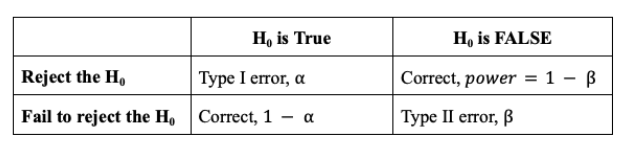
A Type I error, or a false positive, is the error of finding a difference that is not there, so it is the probability of incorrectly rejecting a true null hypothesis is ɑ, where ɑ is the level of significance. It follows that the probability of correctly failing to reject a true null hypothesis is the complement of it, viz. 1 – ɑ. For a particular hypothesis test, if ɑ = 0.05, then its complement would be 0.95 or 95%.

While we are not going to expand on these ideas, we note the following two related probabilities. A Type II error, or false negative, is the probability of failing to reject a false null hypothesis where the probability of a type II error is β and the power is the probability of correctly rejecting a false null hypothesis where power = 1 – β. In common statistical practice, one typically only speaks of the level of significance and the power.

The following table summarizes these ideas, where the column headers refer to what is actually the case, but is unknown. (If the truth or falsity of the null value was truly known, we wouldn’t have to do statistics.)

Hypothesis Tests and Confidence Intervals

Since hypothesis tests and confidence intervals are both methods of statistical inference, then it is reasonable to wonder if they are equivalent in some way. The answer is yes, which means that we can perform hypothesis testing using confidence intervals.

Returning to the example where we have an estimate of the proportion of American men that are avid fans of the NFL, we had (0.40, 0.60) at a 95% confidence level. As a hypothesis test, we could have the alternative hypothesis as H₁ ≠ 0.51. Since the null value of 0.51 lies within the confidence interval, then we would fail to reject the null hypothesis at ɑ = 0.05.

On the other hand, if H₁ ≠ 0.61, then since 0.61 is not in the confidence interval we can reject the null hypothesis at ɑ = 0.05. Note that the confidence level of 95% and the level of significance at ɑ = 0.05 = 5%  are complements, which is the “H_o is True” column in the above table.

In general, one can reject the null hypothesis given a null value and a confidence interval for a two-sided test if the null value is not in the confidence interval where the confidence level and level of significance are complements. For one-sided tests, one can still perform a hypothesis test with the confidence level and null value. Not only is there an added layer of complexity for this equivalence, it is the best practice to perform two-sided hypothesis tests since one is not prejudicing the direction of the alternative.

In this discussion of hypothesis testing and confidence intervals, we not only understand when these two methods of statistical inference can be equivalent, but now have a deeper understanding of statistical significance itself and therefore, statistical inference.

Learn More About Data Science at Flatiron

The curriculum in our Data Science Bootcamp incorporates the latest technologies, including artificial intelligence (AI) tools. Download the syllabus to see what you can learn, or book a 10-minute call with Admissions to learn about full-time and part-time attendance opportunities.

Disclaimer: The information in this blog is current as of February 28, 2024. Current policies, offerings, procedures, and programs may differ.