While most articles focus on deep learning and modeling, as a practicing data scientist you’re probably going to spend much more time finding, accessing, and cleaning up data than you will running models against it.

In this post, you’ll get a quick, hands-on introduction to using the Python “Pandas” library. Whether you’re taking your first steps to becoming a professional data scientist — or just want to save some repetitive work next time you need to clean up a spreadsheet— Pandas is an incredibly powerful tool for easily importing, cleaning, and exporting data.
Pandas envy
It may not be as popular amongst the data science crowd, but as an ex-software developer, Ruby will always hold a special place in my heart. I love the inclusive community, passion for test driving your code, the logical consistency of everything being an object, and the power and comprehensiveness of Rails for building web applications quickly and efficiently.
But ever since I started teaching data science as well as software engineering, I found Ruby lacking in one key area. It simply doesn’t have a fully fledged data analysis gem that can compare to Python’s Pandas library. Usually when I code in Ruby, I appreciate the elegance and economy of expression that the language provides. But after using Pandas for data cleaning, I can honestly say that importing, iterating over, cleaning and then saving data in Ruby is starting to feel a little verbose.
Assumptions
- I’m going to assume that you have a professional data science environment set up on your computer. If you don’t have Python, Jupyter Notebook, and Pandas installed on your machine, here’s one way to get set up for data science.
- I’m also going to assume that you’re comfortable opening up a terminal window and cloning a GitHub repo.
Getting started
Here’s a lab I created for an enterprise project. Start off by opening a terminal window somewhere within your user directory and cloning the repository:
> git clone https://github.com/learn-co-curriculum/ent-ds-del-2-2-cleaning-company-data
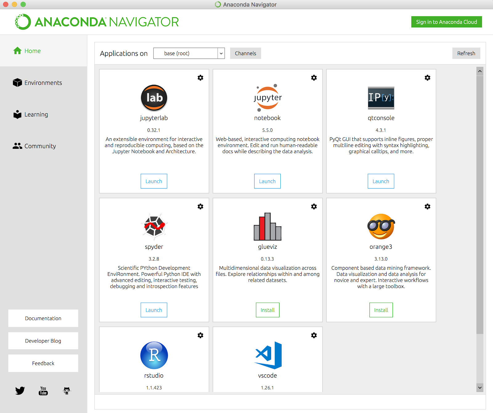
Now start up Jupyter Notebook. If you’re using the Anaconda distribution, run the Anaconda Navigator application and click on the Jupyter Notebook tile to start it up.

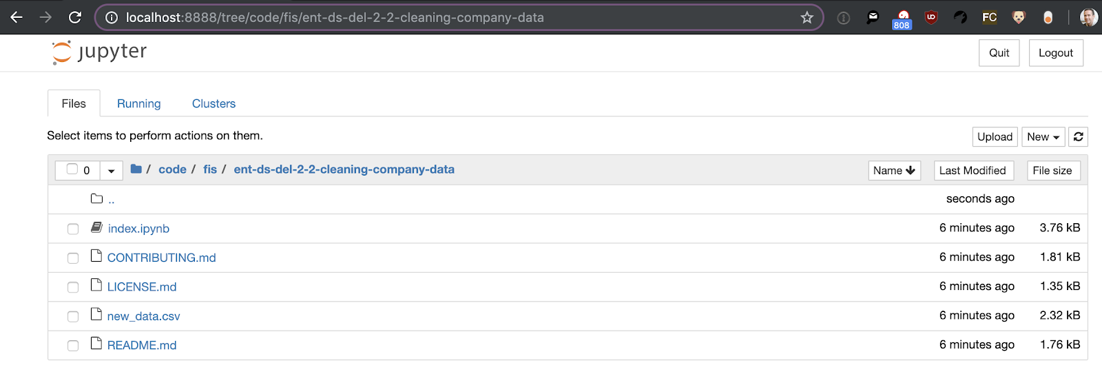
From there, navigate to the directory where you cloned the GitHub repo and you should see an “index.ipynb” file in the directory:

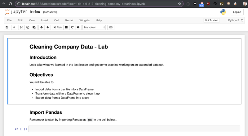
Click on the index.ipynb to open the notebook:

OK, if you haven’t seen a Jupyter Notebook before, it’s rendered in a browser, composed of cells, and a really easy way to intersperse code, comments, charts, and tables. To run code, type it into a “code” cell and hit return. Let’s start by writing and running the boilerplate code to import the Pandas library (as per convention, assigning it to the variable “pd”), remembering to hit “shift-enter” to run the cell.

Importing and exploring data
Let’s see how easy it is to import the “new_data.csv” data into Pandas:

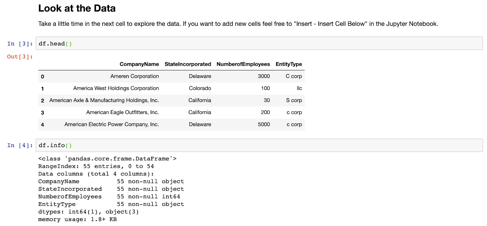
Next up let’s have a quick look at the data, starting with .head() to view the first few rows, and then using the .info() method to get some general information relating to the entire data set:

OK, so it looks like we have a set of company names, the states they were incorporated in, their number of employees, and what kind of legal entity they use. Let’s imagine we wanted to know how many of these companies were of each entity type. Let’s start by using the value_counts() method to learn more about the values within the EntityType field:

OK, so it looks like we’ve got C-corps, S-corps and LLCs, but you can see, due to inconsistent capitalization, it thinks there are six different entity types instead of three. Cool. We’ve imported a data set and learned something about it. Now let’s clean it up.
Cleaning up data
There are lots of ways of making the capitalization consistent for the EntityType – everything from going through manually cleaning up the data to downcasing the entire file to lower case – one character at a time. Let’s see how we could use Pandas to make the capitalization more consistent.
Firstly, let’s just see one way to iterate over a data frame by writing and running the following code:
> for i in df.index:

>    print(df.at[i, 'EntityType'])
And remember, indentation is meaningful in Python, so make sure to indent the line with the print statement to ensure that it’s part of the for-loop.

OK, that seems to be working. Next step, let’s capitalize all of the records using the following code:
> for i in df.index:

>     df.at[i, 'EntityType'] = df.at[i, 'EntityType'].upper()

> df['EntityType'].value_counts()

That’s not bad – we’ve solved the problem in just a few lines of code. But I wonder if we could have done something even slicker by taking advantage of some of the other methods built into Pandas rather than just treating it as a dumb data container to iterate over.
Selectors
One approach would be to use Pandas selectors to apply transformations to a subset of the records without having to iterate. Let’s reload the data into a new data frame and give it a shot:
> df2 = pd.read_csv(new_data.csv')

> df2.loc[df2["EntityType"] == "llc", "EntityType"] = "LLC"

> df2.loc[df2["EntityType"] == "c corp", "EntityType"] = "C corp"

> df2.loc[df2["EntityType"] == "s corp", "EntityType"] = "S corp"

> df2['EntityType'].value_counts()

Exporting data
Finally, once you’re happy with the changes you’ve made, it’s just a one-liner to save the data to a new file, with just two extra lines to read the exported data back in and to confirm it’s saved all of our changes:

Summary
We have only just scratched the surface of what Pandas can do. It really is a Swiss Army knife for exploratory data analysis. The range of methods available can feel overwhelming, but try to get into the habit of using Pandas as your go-to tool for cleaning up spreadsheet data, and then over time you can try out additional methods to expand what you can do with Pandas.


