As a data scientist, a big part of your job is obtaining the data that you need to operate on. In many companies, that data will be stored in one or more relational databases. The goal of this article is to introduce relational databases – what they are and why they’ve historically been so popular.

Different types of data
It’s important to understand that there are different types of data, each of which lends itself to different storage mechanisms. One common, and important, characterization is the distinction between structured and unstructured data.
Structured data is something that would fit really well into a spreadsheet. Think lots of small chunks of information with consistent labels. Addresses, for example, are structured data. Most US addresses comprise of the same five fields – the street address, the second address field (e.g. PO box), the city, the state and the zip code.
Unstructured data is the kind of information you’re more likely to store in a Word or Google doc. A dissertation, a phone call transcription, the contents of a book. Unstructured data doesn’t really break down into small consistent chunks of information that can be usefully separated or queried (as opposed to addresses where you might want to retrieve all the addresses within a given city, state, or zip code).
And then there’s semi-structured data— a mix of structured and unstructured data. If you go to the doctor, they might ask for your first name, last name, weight, and height. That’s all structured information that would fit well in a spreadsheet. But there might also be a large “notes” field with unstructured text describing the doctors observations of your symptoms.
In practice, as you get more items of unstructured data, you can turn them into semi-structured data. If I just write one dissertation, I’m probably going to store it in an unstructured format, like a Google doc. If I’m responsible for reviewing and grading 100 dissertations, I’ll probably treat them as semi-structured data with first name, last name, department, submission date, and grade as some of the structured information and then a link to the PDF submitted to hold the unstructured text of the dissertation itself.
It started with a text file
In the early days of microcomputers, if you wanted to store information to disk, you’d write it to a text file, or if you were feeling ambitious, some kind of more efficient binary storage format. Effectively you were designing your own storage mechanism from scratch every time you wrote a piece of software. If you just wanted to save unstructured data, it was pretty easy. Write it to a file when it changes and read it from the file when you want to get it back.
The problems started when you wanted to work with structured data. You could just write the column names out first and then save the information in a comma or tab separated format. But if you wanted to retrieve a subset of the data (say all the addresses of students living in California), it was inefficient as you had to read through every single record in the file to find the records that you wanted.
For example, if you had a list of 20,000 students and wanted to retrieve the 500 that lived in California, you had to go get all 20,000 students and just discard the ones that weren’t in California. That made retrieval operations very slow — especially for large data sets. It’d be like having a filing cabinet full of student files and having to take out and put back every single one just to find which ones lived in a given state.
Moving to tables
One way to improve that situation was to store the information in two-dimensional tables — think an Excel spreadsheet — with the column names at the top and the data in the rows below it. In itself that doesn’t improve much, but it sets us up to be able to add indexes and they make all the difference.
Adding indexes
In a relational database, you’ll get tables and indexes. Indexes allow you to say “I care about getting information back based on the value of this field, make it faster to do that”. They work by saving additional information (“pointers”) on the hard drive, pointing to the records based on the value of a given field, and they make it very quick to retrieve information based on that value of the indexed field.
For example, if you index a list of mailing addresses by city, the database will take a little more time when saving every new address as it has to write to the index. But, that will make it faster to “retrieve all addresses in San Francisco”. Effectively we’re trading a little loss of write performance (how long it takes to save something) for a substantial improvement in read performance (how long it takes to return a set of records).
This is a particularly good trade off for data that you read more often than you write. For example, optimizing read performance for an article on The New York Times is much more important than optimizing write performance, because any given story is updated just a few times times (assuming there are some edits/corrections) but read hundreds of thousands of times.
Even though they don’t feature prominently in most introductions to relational databases, indexes are actually what made such databases so powerful and performant.
Removing duplication
The name “relational” database comes from the idea of having multiple, related tables. Here’s the theoretical paper underpinning the approach, written by Ted Codd while he was working at IBM in 1970. If you have a few minutes, it’s worth a quick read. Getting into the habit of reading research papers will serve you well as a data scientist and the math in this one is pretty straightforward!
Let’s say we want to create a database of courses and their associated textbooks for a local community college to make it easy for students to find and order the books they need. It might look something like this:

Do you notice the duplication within the table? The most obvious is that the professor name and course name is repeated for every book. Firstly, this wastes hard drive space. That’s not a big deal now, but back in 1970 when you were paying $250 per Mb, it was a real consideration!
More importantly is the risk of error. There’s an important principle in programming called “DRY” – or Don’t Repeat Yourself. The idea is that if you write the same code in multiple places, at some point in time you’re likely to change the code and may forget to change it in one of the locations. The same is true for data. Firstly, you might mistype the data when initially entering it. More importantly, if the data changes in the future (perhaps you change which professor is teaching a course), you might forget to update one of the rows, confusing students because they won’t know which professor is going to be their instructor!
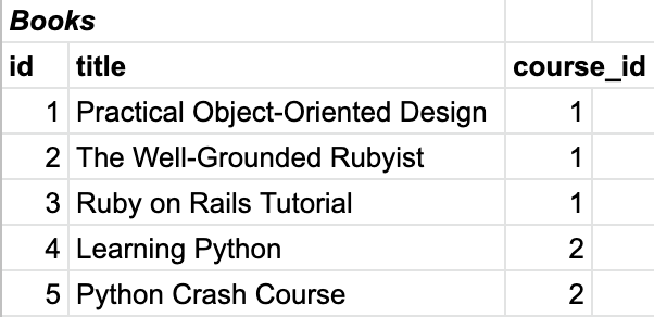
Relational databases solve this problem by supporting multiple, related tables. In this case, we might create one table for the courses and another for the books, with a unique identifier used to “join” the tables.


You can see that, in this case, we’ve used an auto-incrementing integer for the index. That’s just a fancy way of saying that the ID for a given column starts at “1” and increases by 1 for each new record.
ID’s don’t need to be auto-incrementing or integers – they just need to be unique. No two rows in the same table can have the same value for their “primary key” – the field used by the database to uniquely identify rows within that table. In this case, it’s the field we’ve called id.
And you’ll see that in the Books table, we have a course_id field that relates back to the Courses table, so the first three books can be “joined” to the course with an id of 1 – “Introduction to Ruby.” This way, if we have to update the professor associated to a course, we can do it by updating just a single row in the courses table.
And that is the heart of a relational database — using multiple “related” tables to reduce duplication.
Denormalizing a database
Just to cover an edge case that you may come across, we also need to understand how to think about denormalization of relational databases.
One challenge with reducing duplication by splitting information across related tables is that it can affect performance. In general, the more tables your data is split between, the longer it’ll take to retrieve. For most applications, that is a perfectly acceptable trade off, optimizing for the quality and consistency of your data over the speed of a given query, but sometimes such queries are just not fast enough. At that point in time, you might deliberately decide to denormalize your database a little.
For example, if I need to display the comments posted by users on a popular website, I’ll have a comments table for storing the comments and a users table for storing information on the people who commented. But I might also store a copy of the usernames in the comments table so that I don’t have to pay the performance penalty of joining the two tables every time I retrieve the comments.
For a high traffic site, that’s probably not a bad trade off. It will meaningfully improve the performance of a common request (display article comments), and the risk of the data getting messed up is reasonably limited as people generally don’t change their names very often!
Wrapping it up
So, to summarize, relational databases are particularly good at storing and retrieving structured data. The related tables allow you to reduce duplication and the risk of inconsistent data, and the indexes allow you to efficiently retrieve subsets of the data and/or order the data based on one or more of the “fields.”


